Alexandru Mihai — Programming

Finding the optimal strategy for 2048 using Machine Learning

By letting python take control of the keyboard and mouse one can let the computer learn how to play the game 2048 without hard-coding the intricacies of the game itself.

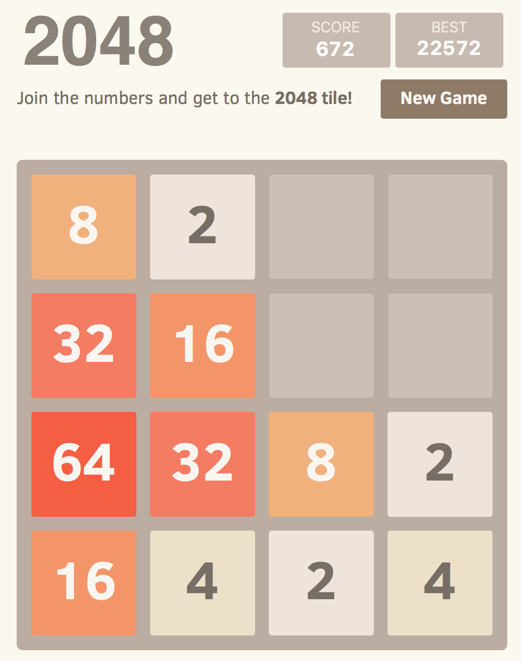
Possible state of 2048 Game

Using the Python packages pyautogui and PIL we investigate the game play of 2048. Gameplay is actuated by pressing one of the arrow keys which shifts the cells seen in Figure 1 in the given direction. An example of the procedure is seen below, the corresponding moves are Down, Left and Down again.

Matrix Form of board

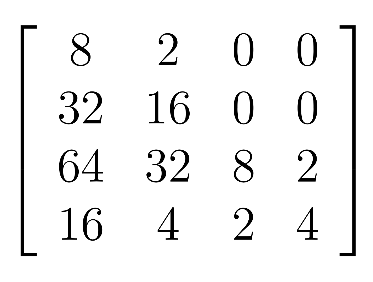
We extract the numbers by finding the pixel color of each square. The ideal strategy of game play can be easily summarized into a Weight matrix. This weight matrix gives us the locations on the board where higher numbers should be as to maximize the long term reward. Throughout my research I found that almost every implementation hoping to beat the game uses some sort of weight matrix to place larger numbers into corresponding patterns, when possible that is.

After playing the game a few times one may notice that we prefer the largest number to be located in a corner, but what of the second largest and the third largest? The interesting result is that the weight matrix is not symmetric. An example of a weight matrix found by Yiyuan Lee is seen below.

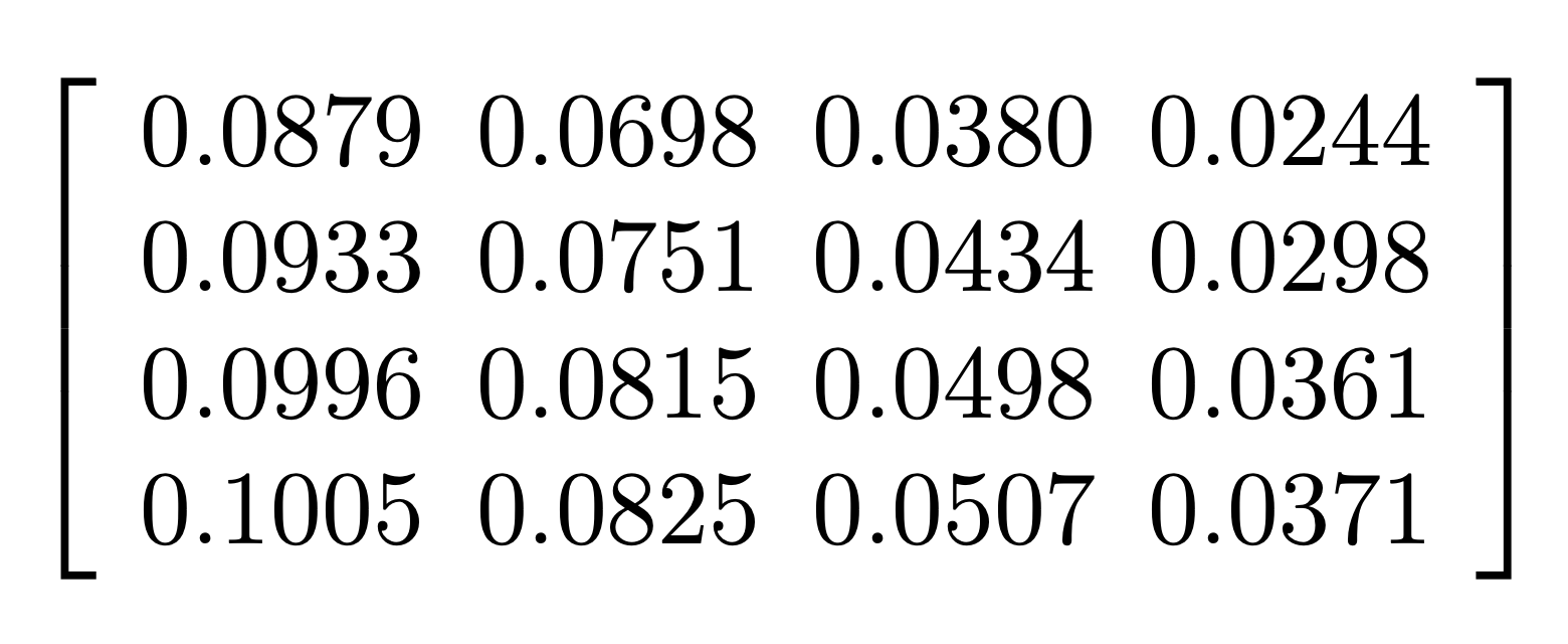
Notice how the largest weight is found in the top right corner with progressively smaller weights found along columns. Instead of working with the entirely of the state space of 2048 we limit our algorithm to the first 13 moves. This allows us to compute the Q-Values with respect to the next state by setting our state to be the move number. This gives us a Q-Value matrix of 13 by 4 due to the four possible actions. After some mathematical manipulations and many, many hours of my computer playing the game we can also recover a weight matrix.

The process described above maintains the total sum of the weights at 1, as such the result is slightly different from the weight matrix given above. But the geometric relationship of the weights is recovered. Also considering the symmerty of the system. This asymmetric and non-intuitive result is what we interpret as the optimal strategy of the game 2048. A more detailed description with a bit more math can be found at 2048 Q-Learning

Computational Fluid Dynamics

The majority of work seen here was completed as part of my Guided Research at Jacobs University in Bremen, in collaboration with the Fraunhofer MEVIS Institute, as a part of my Batchelor's Disertation.

Lattice Boltzmann Method implementation in 2D

For this project I implementated what is refered to as a mesoscopic method of simulation. While the typical Finite element methods are considered macroscopic and methods resembeling older algorithms like Lattice Gas Automata are microscopic. Meaning that the Lattice Boltzmann Method focuses neither on the microscopic world of molecules, nor the continuous world of pressure and velocities. It is somewhere in-between.

One of the advantages of the Lattice Boltzmann Method is it ease of dealing with any geometry and its parallelizability. As such it was applied to a system which requires high accuracy and the geometries are not simple, Blood Flow dynamics. First, the I hardcoded the discretization and the algorithm for a two dimensional geometry. A channel with two bumps on either side to simulate a narrowing, or stenosis of a blood vessel.

Velocity and pressure plots in a 2D stenotic geometry at a Reynolds number of 714 after 480 iterations.

Velocity and pressure plots in a 2D stenotic geometry at a Reynolds number of 1429(higher inflow velocity) after 480 iterations.

Notice that as the inlet velocity increases a periodic pattern develops in the flow. This could be an example of the transition between laminar flow and turbulent flow. It also has medical significance, if this really were a blood vessel then the fact that the pressure drop before and after the narrowing is not constant should be taken into account when treatments are considered.

More typical Streamline plots can also be generated of course.

OpenLB and 3D Blood Flow Simulations

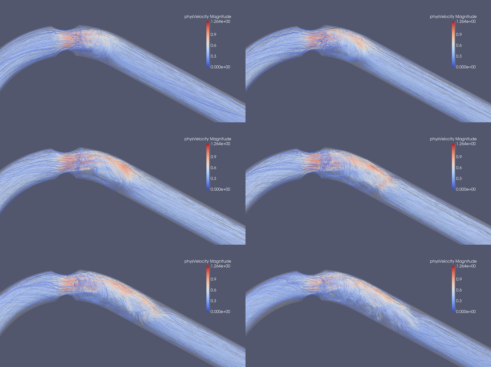
With the aid of the open source library OpenLB developed by Mathias J. Krause of the Karlsruhe Institute of Technology, simulations similar to those seen below were produced to analyze the stability of blood flow through a stenotic aortic geometry.

Flow through a cylindrical geometry with a narrow section.

A simplification of a human aorta with a narrowing following the arch.

Airfoil Simulations

This was only a simple experiment to test the boundaries of my code in 2D. The flow is not as of yet stable due to blow up near the trailing edge. Above is the velocity of the flow and below it is the pressure throughout the domain.

Additional Coding Projects

Simulating Capillarity with Smooth Particle Hydrodynamics

Using the smooth particle hydrodynamics(SPH) framework, simulations of a free surface inteacting with non-trivial geometries are investigated. The SPH method is a Lagrangian particle method originally used for astrophysical simulations. Monaghan [6] first described a possible implementation of the method to model incompressible fluids with complex geometries and since then it has grown significantly. The simulations were run with the aid of the PySPH open source library.

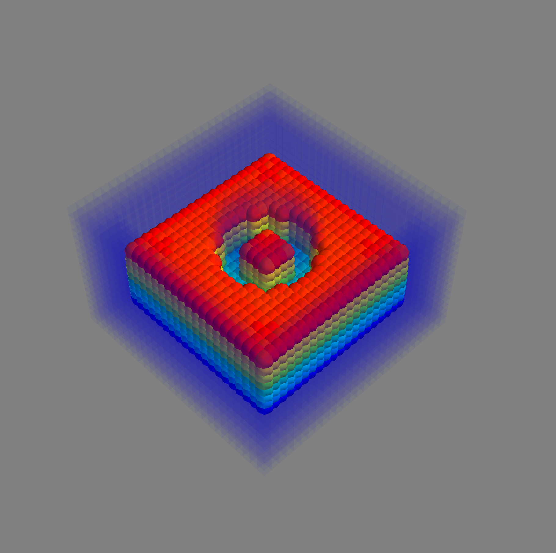
2D simulations of a capillary tube with 12796 fluid and 6126 solid particles. The left shows the 100th iteration and the right an equilibrium state after 80,000 iterations. Particles are colored by pressure.

3D simulations of a capillary tube with 2944 fluid and 7769 solid particles. The left shows the initial configuration and the right an equilibrium after 18,000 iterations. Particles are colored by height(z-coordinate).

As the initial state of the fluid particles is a non-physical lattice arrangement the simulation must reach an equilibrium, seen in the images on the right. Interestingly this transition to equilibrium can be viewed as a numerical equivalent of analytic variational principles used to model the system.

Modeling Distribution Networks using the Nagel-Schreckenberg Traffic Model and Varying Junction Rules

At the heart of the wide and diverse field of Logistics lies the transport of goods. This transport occurs at a multitude of scales and between multiple locations of varying distances. The theory of traffic simulation has been thoroughly investigated, for example by Wolfram and his Rule 184 of cellular automata, as well as by the famous Nagel-Schreckenberg model.

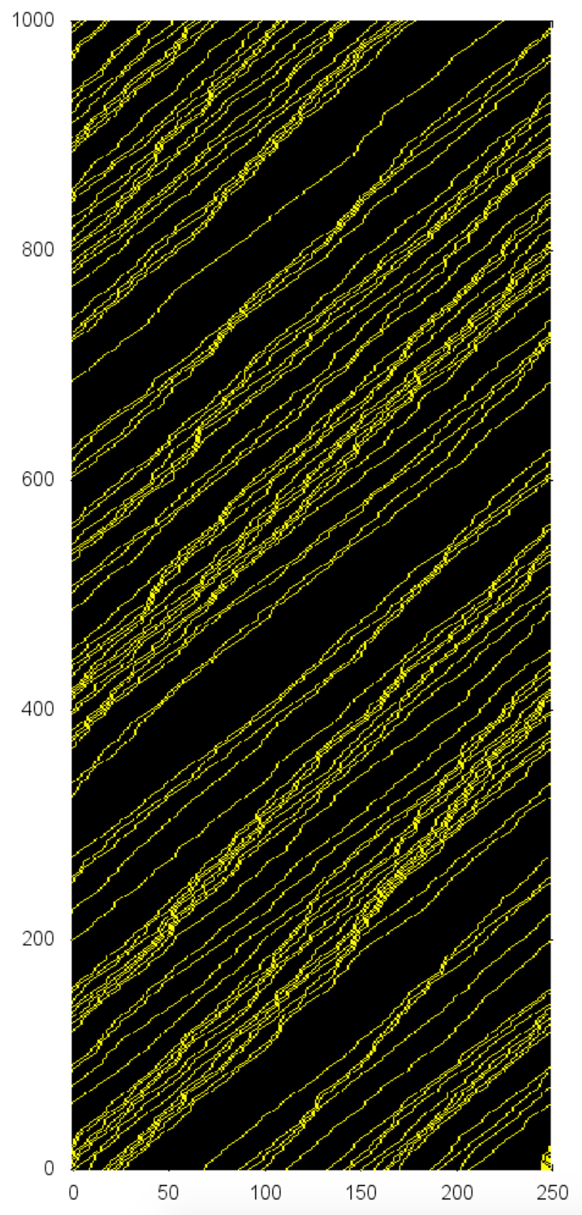
Two simulations were produced using the Nagel-Schreckenberg model with varying probabilities (0.3 on the left, and 0.75 on the right) that the vehicle will slow down without reason(Dawdle Probability). The horizontal axes represent the space domain while the vertical axes show the change in the systems with respect to time.

The aggregation of cars, here depicted as yellow pixels, is due to the Braking/Dawdle Probability described above. The reason the plot on the left has a larger build-up of cars, or a traffic jam, is specifically because its Braking Probability is much greater. These plots as essentially detailing the traffic between 2 nodes, meaning with the addition of some junction rules we can consider the traffic on a directed graph or network.

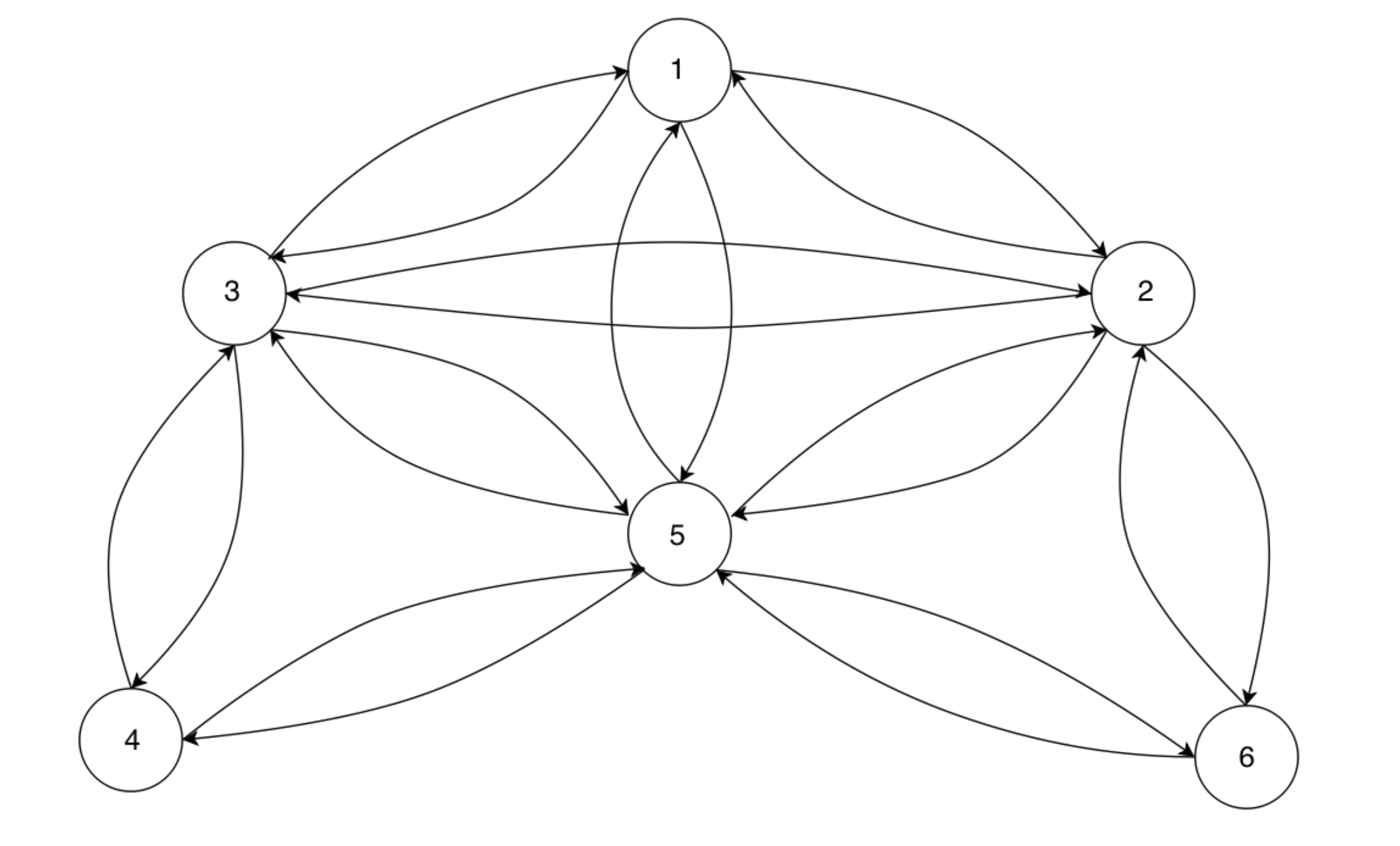
There are 20 streets in total. Because this is a directed graph one will notice that cycles are easily found.

These cycles could be interpreted as the areas where cars will travel, there could be an even distribution, whereas cars are distributed to random streets the moment they reach a node, or a fixed rotary junction where each given street is forced to go to pair according to the cycle. Firstly, we are interested in a cycle which contains all streets. Because of the parity of the network we are able to find such a cycle. Using the labels we can explicitly define the order of nodes that a car would pass through. That order is: 1→2→6→5→4→3→1→5→6→2→5→3→4→5→1→3→2→3→5→2→1.

With this order we can simply connect the Space-Time plot of each street with the next one in the order. While this is only one order out of many possibilities it should be representative.

Simulations carried out with a Braking Probability of 50% and Density of 50%

The rotary junction forces each car to follow the order of the streets that was determined above. The Random junction chooses a random street once the car reachs a node. Lastly, I implemented a junction rule that combines the original two approaches. This mixed junction rule implements a randomized junction at the node with the highest degree of connectivity, and creates small cycles of three nodes with the rest of the streets. Namely, it creates cycles between nodes 1, 2, and 3 as well as nodes 3, 4, and 5 and lastly nodes 2, 5, 6 are also connected.

More results and detailed explinations can be found here. And the code used to generate the images in this section is here.(Note gnuplot needed for actual pictures.)

Clustering Data using the continuous solution to the Heat Equation

While supervising the Graph Spectral Clustering reasearch group at the Summer@ICERM program I relized that most data clustering algorithims use discritized versions of mathematical functions or algorithims. This makes sense as data is usually inherently discrete. But as a proof of concept what if we could make discrete data continuous in some way such that we could potentially select groups of such data from the solution of a continuous system?

The clustering algorithm I propose is not even an algorithm, it is a function. A function which takes points in the plane as inputs, and it outputs either centroids of the data, or contours corresponding to those centroids. Graph spectral clustering uses a discretized version of the Laplace operator, meaning that instead of a differential Equation one has a matrix equation, which is rather simple for a computer to deal with. But the Laplace operator itself is a very common part of differential equations. So common and simple that for many forms of the Heat equation(which is based on the Laplace operator) can be solved completely given a simple doimain.

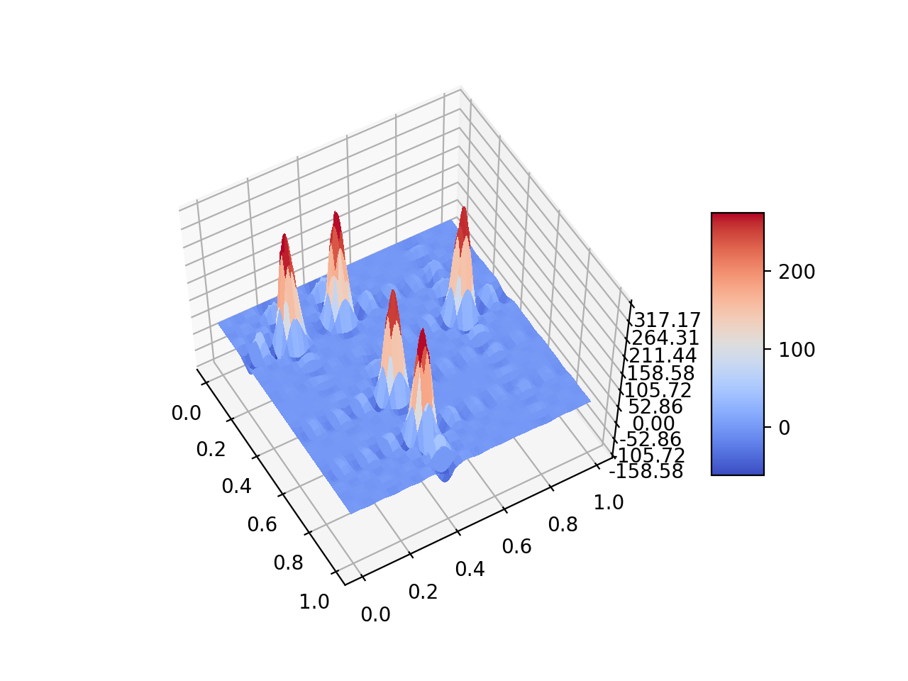
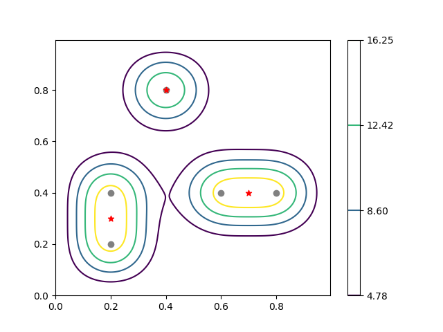
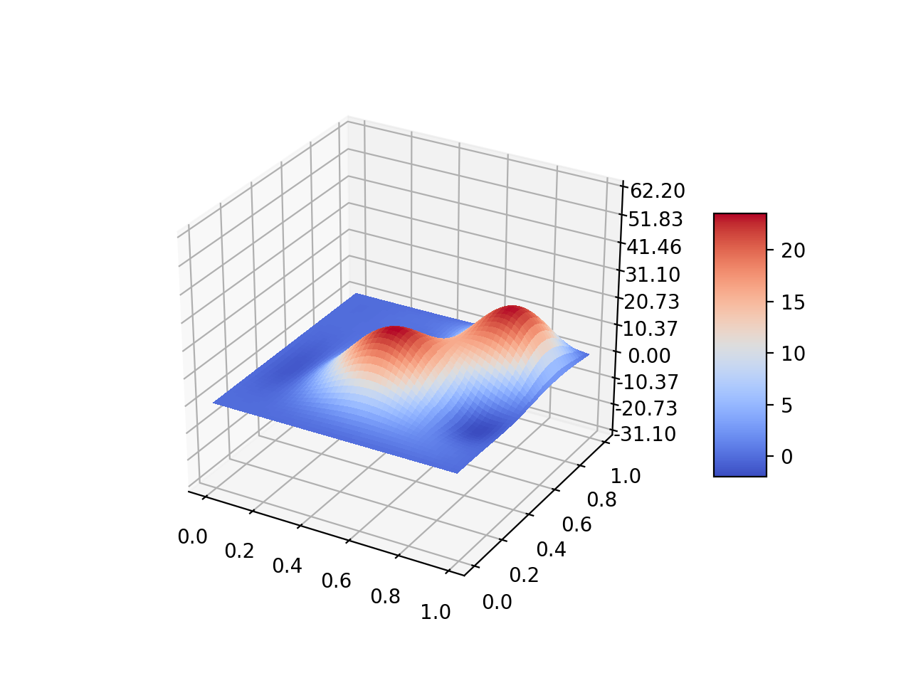
And this was the fact that I took advantage of, turning points in the plane into distributions, which can in turn be used as initial conditions for the Heat Equation in two dimensions. From this point, we have a differential equation, a domain, and an initial condition. Meaning that this system can be solved. Given an initial condition consisting of two dimensions the solution will be a surface. By finding the peaks of this surface we find that they correspond with the centroids that are recovered by a typical K-Means clustering algorithm. Not only that but as we vary the "time" at which to eveluate the solution we can recover any number of centroids. This is because of the nature of the boundary conditions and that "heat" dissapates, meaning that the clusters found at a later relative time will contain more and more of the initial points. Interactive applet and mathematical derivation coming soon...

Solution of the function at a very small "time".

Solution of the function at a relatively bigger "time".